Light Curve Tool for Small Bodies

Introduction

This application is specifically designed to generate light curves for small, atmosphere-less bodies in the Solar System, with the primary objective of supporting research in this domain. While alternative tools exist, this application offers a distinctive combination of features: simulations are executed directly on the server, eliminating the need for local installation, and it generates projected images of objects in the sky plane. These functionalities are particularly valuable for validating research in fields such as stellar occultations. Developed in Python with Django as its framework, the tool currently provides two operational modes specifically designed for photometric studies of rotational lightcurves—the Known and Generic modes—as well as an additional Occultation mode for stellar occultations.

• Known Body Mode: Allows users to generate the light curve and projected shape of a known object by entering its Minor Planet designation and observation date.
• Generic Body Mode: Enables users to perform generic simulations of an object by specifying its aspect angle.
• Occultation Mode: Computes the projected silhouette of a body at the epoch of a predicted stellar occultation, allowing direct comparison with observed chords.

In all modes, users have the option to upload a custom shape model in .obj format or define the triaxial axes (a, b, and c) of an ellipsoid. Both the shape model dimensions and the axes are assumed in kilometers.

The following sections provide a detailed explanation of each tool's features. For a demonstration of its functionality, watch this video. A complete description of the tool, including usage examples and validation tests, is available in the accompanying research paper: Rizos et al. (2025), Astronomy & Astrophysics.

Known Body Mode

Object: In this mode, the user is required to provide the Minor Planet number assigned to the object. This information can be retrieved from the JPL Small-Body Database.

Date: The user must also specify the observation date from which the light curve should be simulated. The required format is yyyy-mm-dd hh:mm:ss.ssss (e.g., 2001-01-01 12:30:12.4320). If the date provided is in the yyyy-mm-dd format, the tool will automatically assume the time to be 00:00:00.0000.
The viewing geometry is fixed to the date specified by the user, independent of the rotation period length. In extreme cases where the period is so long that the geometry changes significantly over a single rotation, we recommend using the Generic Mode (described below) and adapting the settings to the specific problem.

Rotation Pole: For known bodies, the rotation pole must be specified in ecliptic coordinates, using decimal degrees. Longitude is defined in the range 0–360°, and latitude in the range –90° to +90°. If the pole coordinates are known in a different reference frame, you can convert them using this external tool. Once defined, the rotation sense follows the right-hand rule.

Generic Body Mode

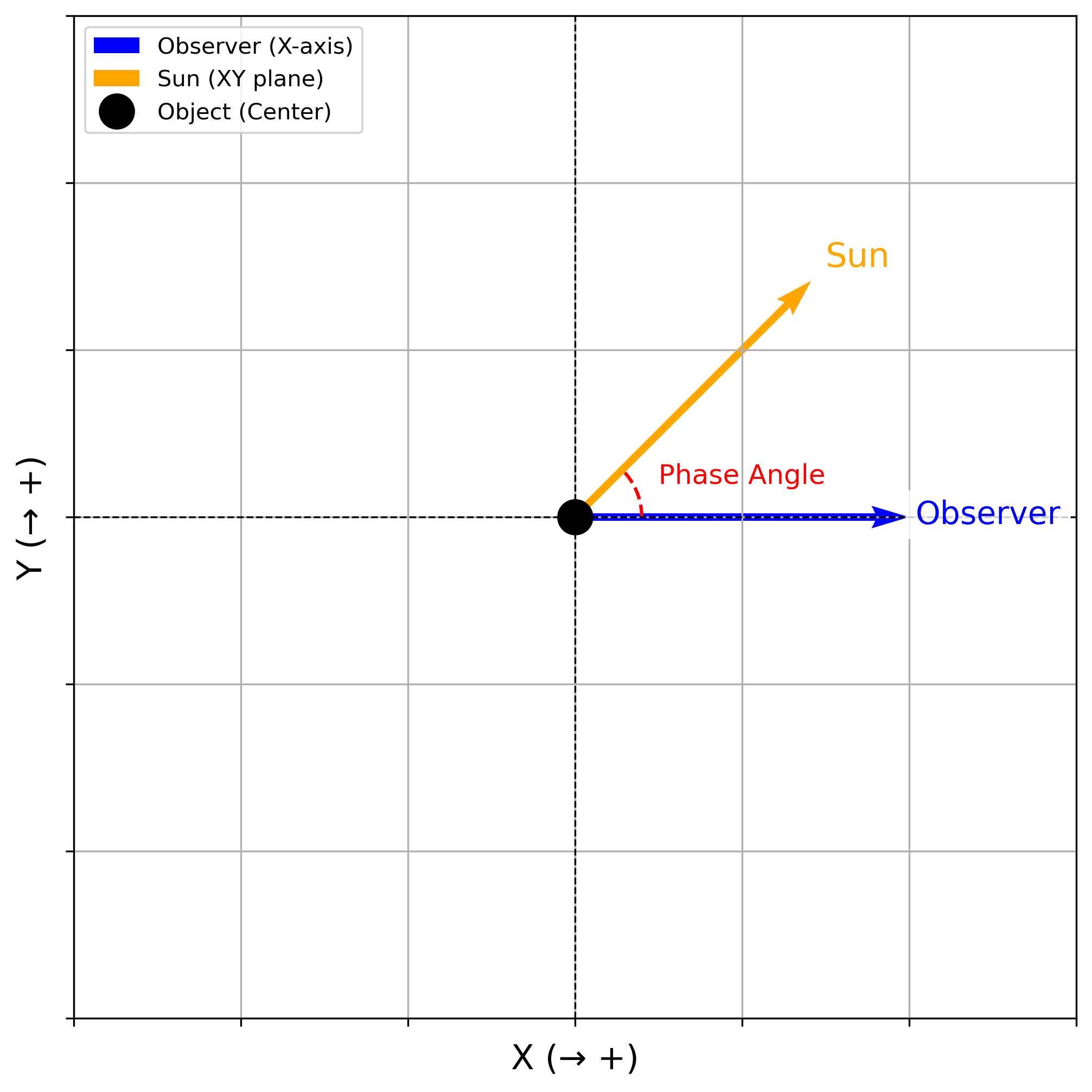
Phase Angle: The phase angle is the angle formed between the vector pointing toward the Sun and the vector pointing toward the observer. In this mode, Earth (observer) is fixed along the X-axis of this arbitrary coordinate system, the object is located at the origin, and the Sun moves according to the angle specified by the user within the XY plane (from the X-axis toward the Y-axis, see Fig. 1). In case the check box Generate Images is selected, the positive Z-axis points upward, while the positive Y-axis is oriented to the right in the image.

Rotation Pole: In this mode, Earth (observer) is fixed at the origin and lies on the XY plane, with Y = 0, as illustrated in Fig. 1. The pole is defined using spherical coordinates in this arbitrary frame. A pole at longitude = 0° and latitude = 90° corresponds to an "equator-on" configuration, while a pole at longitude = 0° and latitude = 0° corresponds to a "pole-on" configuration. Once defined, the rotation sense follows the right-hand rule.

Common Input Parameters for the Rotational Light Curves

LC number of points: This parameter defines the temporal resolution of the rotational light curve. It specifies the number of points sampled across one full rotation. The tool currently supports up to 360 points, corresponding to 1° phase increments. For exceptional cases requiring higher resolution, please contact the developer.

Rotational phase offset: A rotational phase offset, ranging between 0 and 1, can be applied to adjust the starting point of the light curve. This adjustment ensures that the curve begins at a specific phase, such as a maximum, minimum, or any other desired point.

Shape Model

Custom Shape Model: A custom shape model can be uploaded in .obj format, with facets required to be triangular for compatibility. It is recommended to use Blender, a free and versatile software, to create and export models in the appropriate format for this tool. Models with a higher number of facets will result in longer computation times, and it is recommended not to exceed 3000 facets. In this video, the user can find a basic example of how to generate a shape model. It is important to specify that the forward axis is set to Y and the up axis is set to Z before exporting. Otherwise, an undesired orientation may occur. An example of a shape model in the required format can be downloaded at this link.

Triaxial Ellipsoid: A triaxial ellipsoid composed of 642 triangular facets can be generated by specifying the values of the axes a, b, and c. The shape model generated through this process will be included in the download folder.

Photometric Model

Radiance represents the intrinsic brightness of an object, independent of the observation distance or measurement instrument, but dependent on the photometric angles of phase (α), emission (e), and incidence (i). It is quantified as energy per unit area, solid angle, and time. However, for small bodies reflecting sunlight, it is often more practical to consider the ratio between incident and reflected energy. A commonly used term for this is I/F, which represents the ratio of reflected light to that of a perfectly Lambertian surface under the same illumination conditions. In this tool, several photometric models are implemented. On the one hand, we use empirical models, assuming that radiance can be expressed as the product of two components: a phase function (f(α)) and a disk function (d(α,e,i)). This approach allows the simulation to separately account for the effects of the Sun-object-observer geometry (phase angle) and the surface scattering properties of the object.

$$\frac{I}{F} = f(\alpha) \; d(\alpha, e, i)$$

On the other hand, we implement the Hapke model (Hapke 2012). This model is significantly more complex than empirical models but has the advantage that its parameters have a physical meaning (or at least that's what it's supposed to be), making them more intuitive and applicable in scientific studies.

For simplicity, the solar irradiance (S) received by the object is normalized to 1 W/m². This assumption facilitates rescaling of the results if needed.

The currently implemented and functional models are as follows:

Empirical models:

Phase functions

• No phase function: Assumes no dependence on the phase angle:
  
  $$f(\alpha) = 1$$
  
  
• Minnaert: Assumes a dependence as follows:
  
  $$ f(\alpha) = A_{\text{min}} \; \pi \; 10^{-0.4 (\beta \alpha + \gamma \alpha^2 + \delta \alpha^3)} $$
  
  where Amin, β, γ, and δ are fitting parameters (these parameters must be derived using degrees,not radians).

Disk functions

• Lambertian: Assumes isotropic scattering given by:
  
  $$d(i) = \frac{\cos i}{\pi}$$
  
  
• Lommel-Seeliger: Models as:
  
  $$ d(e, i) = \frac{\cos i}{\cos i + \cos e} $$
  
  
• Minnaert: Dependence on incidence and emission, parameterized through the parameter k:
  
  $$ d(e, i) = \cos^k (i) \; \cos^{k-1} (e) $$
  
  

Hapke model:

The Hapke model is based on radiative transfer theory and provides a more intuitive and interpretable approach to surface scattering. The model accounts for multiple scattering, macroscopic roughness, and opposition effects, which improve the accuracy of brightness predictions for irregular and granular surfaces. The reflectance in the Hapke model used in this tool, which depends on 9 parameters, is given by:

$$ \frac{I}{F} = LS(i, e) \; K \; \frac{w}{4} \left[ p(\alpha)(1 + B_{S0} B_{S}(\alpha)) + M(i, e) \right] \left[ 1 + B_{C0} B_{C}(\alpha) \right] S(i, e, \psi) $$

where:

• LS(e, i) is the Lommel-Seeliger function.
• K is the porosity factor, accounting for voids between particles in the surface.
• w is the single-scattering albedo, representing the fraction of incident light scattered by a single particle.
• p(α) is the phase function.
• BS0 is the amplitude of the Shadow Hiding Opposition Effect (SHOE).
• BS(g) is the SHOE function.
• M(i,e) is the Isotropic Multiple-Scattering Approximation (IMSA).
• BC0 is the amplitude of the Coherent Backscatter Opposition Effect (CBOE).
• BC(α) is the CBOE function.
• S(e, i, ψ) represents the macroscopic roughness correction, accounting for large-scale variations in the surface slope, where ψ is the azimuthal angle between the planes of incidence and emission:

$$ \psi = \arccos \left( \frac{\cos(α) - \cos(e) \cos(i)}{\sin(e) \sin(i)} \right) $$

Each term of the above equation is calculated as:

• Lommel-Seeliger function (LS(e, i)):

  $$LS(e, i) = \frac{\cos i}{\cos i + \cos e}$$

• Porosity factor (K):

  $$ K = \frac{-\ln (1 - 1.209\phi^{2/3})}{1.209\phi^{2/3}} $$

  where Φ is the filling factor, equivalent to 1 - porosity.


• Phase function (p(α)), we employ the Henyey-Greenstein double-lobed single particle phase function:

  $$ p(α) = \frac{(1 + c_{HG})}{2} \; \frac{(1 - b_{HG}^2)}{(1 - 2b_{HG} \cos α + b_{HG}^2)^{3/2}} + \frac{(1 - c_{HG})}{2} \; \frac{(1 - b_{HG}^2)}{(1 + 2b_{HG} \cos α + b_{HG}^2)^{3/2}} $$

  
  where bHG (0 ≤ bHG ≤ 1) is the shape-controlling parameter, and cHG (−1 ≤ cHG ≤ 1)is the relative strength of backward and forward lobes.


• SHOE function, or Shadow Hiding Opposition Effect:

  $$ B_S(α) = \frac{1}{1 + \tan(α/2)/h_S} $$

  where hS is the angular width parameter of SHOE.


• Isotropic Multiple-Scattering Approximation (IMSA):

  $$ M(i, e) = H\left(\frac{\cos(i)}{K}, w\right) H\left(\frac{\cos(e)}{K}, w\right) - 1 $$

  where H(x,w) is the Ambartsumian-Chandrasekhar H function, which can be approximated as:

  $$ H(x, w) \approx \left\{ 1 - w x \left[ r_0 + \frac{1 - 2 r_0 x}{2} \ln \left(\frac{1 + x}{x}\right) \right] \right\}^{-1} $$

  where r0 is the diffusive reflectance, given by

  $$ r_0 = \frac{1 - \sqrt{1 - w}}{1 + \sqrt{1 - w}} $$

• Coherent Backscatter Opposition Effect function:

  $$ B_C(\alpha) = \frac{1 + \frac{1 - \exp(-\tan(\alpha/2) / h_C)}{\tan(\alpha/2) / h_C}}{2 \left[ 1 + \tan(\alpha/2) / h_C \right]^2} $$

  where hC is the angular width of CBOE.


• Shadowing function \( S(i, e, \psi) \), which is function of θp, the effective value of the photometric roughness, and given by:
  if i ≤ e :

  $$ S(i, e, \psi) = \frac{\mu}{\eta(e)} \frac{\mu_0}{\eta(i)} \frac{\chi({\theta}_p)}{1 - f(\psi) + f(\psi) \chi({\theta}_p) [\mu_0 / \eta(i)]} $$

  with

  $$ \mu_{0} = \chi({\theta}_p) \left[ \cos(i) + \sin(i) \tan({\theta}_p) \frac{\cos(\psi) E_2(e) + \sin^2(\psi/2) E_2(i)}{2 - E_1(e) - (\psi/\pi) E_1(i)} \right] $$

  $$ \mu = \chi({\theta}_p) \left[ \cos(e) + \sin(e) \tan({\theta}_p) \frac{E_2(e) - \sin^2(\psi/2) E_2(i)}{2 - E_1(i) - (\psi/\pi) E_1(i)} \right] $$

  if e < i :

  $$ S(i, e, \psi) = \frac{\mu}{\eta(e)} \frac{\mu_0}{\eta(i)} \frac{\chi({\theta}_p)}{1 - f(\psi) + f(\psi) \chi({\theta}_p) [\mu / \eta(e)]} $$

  with

  $$ \mu_{0} = \chi({\theta}_p) \left[ \cos(i) + \sin(i) \tan({\theta}_p) \frac{E_2(i) - \sin^2(\psi/2) E_2(e)}{2 - E_1(i) - (\psi/\pi) E_1(e)} \right] $$

  $$ \mu = \chi({\theta}_p) \left[ \cos(e) + \sin(e) \tan({\theta}_p) \frac{\cos(\psi) E_2(i) + \sin^2(\psi/2) E_2(e)}{2 - E_1(i) - (\psi/\pi) E_1(e)} \right] $$

  With the following expressions, which are independent of e and i values, as follows:

  $$ \chi({\theta}_p) = \frac{1}{\sqrt{1 + \pi \tan^2({\theta}_p)}} $$

  $$ \eta(y) = \chi({\theta}_p) \left[ \cos(y) + \sin(y) \tan({\theta}_p) \frac{E_2(y)}{2 - E_1(y)} \right] $$

  $$ E_1(y) = \exp \left[ -\frac{2}{\pi} \cot({\theta}_p) \cot(y) \right] $$

  $$ E_2(y) = \exp \left[ -\frac{1}{\pi} \cot^2({\theta}_p) \cot^2(y) \right] $$

  $$ f(\psi) = \exp \left[ -2 \tan \left( \frac{\psi}{2} \right) \right] $$

To use the Hapke model in this tool, the following 9 parameters are required:

Albedo Spot

The Albedo Spot checkbox allows users to simulate surface features with different reflectance properties (albedo) on the surface. This feature is particularly useful for studying the effects of localized surface variations on the rotational light curve.

When this checkbox is enabled, the user can define the following parameters:

• Albedo variation (%): Specifies the percentage reduction in reflectance for the selected spot. For example, a value of 20% reduces the reflectance by 20% compared to the surrounding surface.
• Latitude range: Defines the minimum and maximum latitudes (in decimal degrees) where the albedo spot is located.
• Longitude range: Defines the minimum and maximum longitudes (in decimal degrees) where the albedo spot is located.

By adjusting these parameters, users can model and analyze how surface heterogeneities influence the rotational light curve of the object.

Precession

The Precession checkbox allows users to simulate the motion of the rotation pole as it precesses over time. Instead of remaining fixed, the rotation pole follows a conical trajectory, modifying its longitude and latitude dynamically during the simulation.

When this checkbox is enabled, the user can define the following parameters:

• Amplitude Lat (°): The maximum variation of the rotation pole's latitude due to precession. A higher value results in a more pronounced inclination change.
• Amplitude Lon (°): The maximum variation of the rotation pole's longitude due to precession. This determines how much the pole drifts in the longitude direction.
• Precession freq. (cycles per body rotation): Defines how many full precession cycles occur per complete rotation of the body. A frequency of 1 means the pole completes one full precession cycle for every full rotation.

The precession is modeled using sinusoidal variations for both the longitude and co-latitude of the pole:

$$ \text{lon} = \text{lon}_{0} + A_{\text{lon}} \; \cos\!\left( 2\pi \, \omega_{p} \, t \right) $$

$$ \text{colat} = \text{colat}_{0} + A_{\text{colat}} \; \sin\!\left( 2\pi \, \omega_{p} \, t \right) $$

Where:

• lon0 and colat0 are the initial longitude and colatitude of the pole.
• Alon and Acolat define the amplitude of the precession in longitude and colatitude .
• ωp is the precession frequency in cycles per body rotation.
• t represents the rotational phase, varying from 0 to 1 over a full rotation.

By adjusting these parameters, users can simulate different precession behaviors, from small oscillations to large variations where the rotation pole traces a wide circular path over time.

Check Boxes

The tool includes the following checkboxes to customize the output:

• Generate Images: Enables the generation of projected images for the object in addition to the light curve. These images can be used for visualization or further validation purposes.
• Self-shadowing: Includes the effect of self-shadowing in the simulation, which considers how different parts of the object's surface may block sunlight. Be aware that enabling this option can significantly increase computation time.

Output

The web interface provides a complete summary of all the parameters used in each simulation.

If the Generate Images checkbox is selected or the Known and Generic modes, an animated GIF is displayed showing the projected shape of the object on the sky plane. For the Occultation mode, the interface also displays the rotational phase of the object at the inserted occultation date, along with the corresponding projected figure.

The colors of the surface facets reflect the solar incidence angle, with red indicating lower values (more irradiated areas) and blue indicating higher ones. The white arrow corresponds to the orientation of the rotation pole at the time of the observation. A scale bar is shown in the bottom-right corner, and the default units of the tool are kilometers.

In the Known and Generic modes, the synthetic light curve in relative magnitude is also displayed, computed as:

where RADF is the sum of the radiance factor from all facets at a given rotational phase, and RADF is the average radiance factor.

By clicking the Download Files button, a ZIP archive is generated and downloaded to the user’s local machine. This archive contains:

• All generated projection images, each named with the corresponding rotational phase.
• The synthetic light curve as synthetic_LC.png.
• The shape model in .obj format (if axes a, b, and c were provided).
• The animated projection GIF (when Generate Images was selected).
• A plain text file named output.dat with the computed numerical results:
  • Column 1: rotational phase
  • Column 2: RADF
  • Column 3: relative magnitude (as defined above)

Similarly, in the case of the Occultation mode, the user can download a ZIP file containing the projected image for the occultation date, the shape model in .obj format, and the output.dat file with all the data corresponding to this case.

Acknowledgements

Rizos, J. L., Ortiz, J. L., Gutiérrez, P. J., Navajas, I. M., & Lara, L. M. (2025).
An open-access web tool for light curve simulation and analysis of small Solar System objects.
Astronomy & Astrophysics. https://doi.org/10.1051/0004-6361/202556525

@article{Rizos2025,
  author  = {Rizos, J. L. and Ortiz, J. L. and Guti{\'e}rrez, P. J. and Navajas, I. M. and Lara, L. M.},
  title   = {An open-access web tool for light curve simulation and analysis of small Solar System objects},
  journal = {Astronomy \& Astrophysics},
  year    = {2025},
  doi     = {10.1051/0004-6361/202556525},
}